Radar Target Classification (Competition)
2020
This project started in 2020.
This project is a competition by MAFAT’s DDR&D (Directorate of Defense Research & Development) that tackles the challenge of classifying living, non-rigid objects detected by Doppler-pulse radar systems using AI. During this competition, I used many data science and machine learning technologies (mainly in Python & MATLAB) and signal processing technics like: - Creating new data for additional training data from new and unfamiliar data format.
- Balancing and partitioning large data with many different strategies for good training and validation sets.
- Using FFT, windows, noise filtering, noise inducing and other techniques.
- Utilizing microphysical effects like micro-Doppler effects to get an edge.
- Creating spectrograms with emphasized important data parts for better results with CNNs.
- Creating light and robust CNN models to be able to run big data on a small GPU memory.
- Reconstructing modified successful models from articles and combine them into one great model that includes CNNs, RNNs and other model types.
The full details are just below.
MAFAT Radar Challenge
Introduction
This competition by MAFAT’s DDR&D (Directorate of Defense Research & Development) tackles the challenge of classifying living, non-rigid objects detected by doppler-pulse radar systems. The competition was divided into two stages, where the first stage was mainly for training and the second stage for testing. This challenge had over 1K participants. You can view the competition site here.
The Radar
The type of radar the data comes from is called a Pulse-Doppler Radar. A Pulse-Doppler Radar is a radar system that determines the range to a target using pulse-timing techniques and uses the Doppler effect of the returned signal to determine the target object’s velocity.
Each radar “stares” at a fixed, wide area of interest. Whenever an animal or a human moves within the radar’s covered area, it is detected and tracked. The dataset contains records of those tracks. The tracks in the dataset are split into 32 time-unit segments. Each record in the dataset represents a single segment.
A segment consists of a matrix with I/Q values and metadata. The matrix of each segment has a size of 32x128. The X-axis represents the pulse transmission time, also known as “slow-time”. The Y-axis represents the reception time of signals with respect to pulse transmission time divided into 128 equal sized bins, also known as “fast-time”. The Y-axis is usually referred to as “range” or “velocity” as wave propagation depends on the speed of light.
The radar’s raw, original received signal is a wave defined by amplitude, frequency, and phase. Frequency and phase are treated as a single-phase parameter. Amplitude and phase are represented in polar coordinates relative to the transmitted burst/wave.
Upon reception, the raw data is converted to cartesian coordinates, i.e., I/Q values. The values in the matrix are complex numbers: I represents the real part, and Q represents the imaginary part.
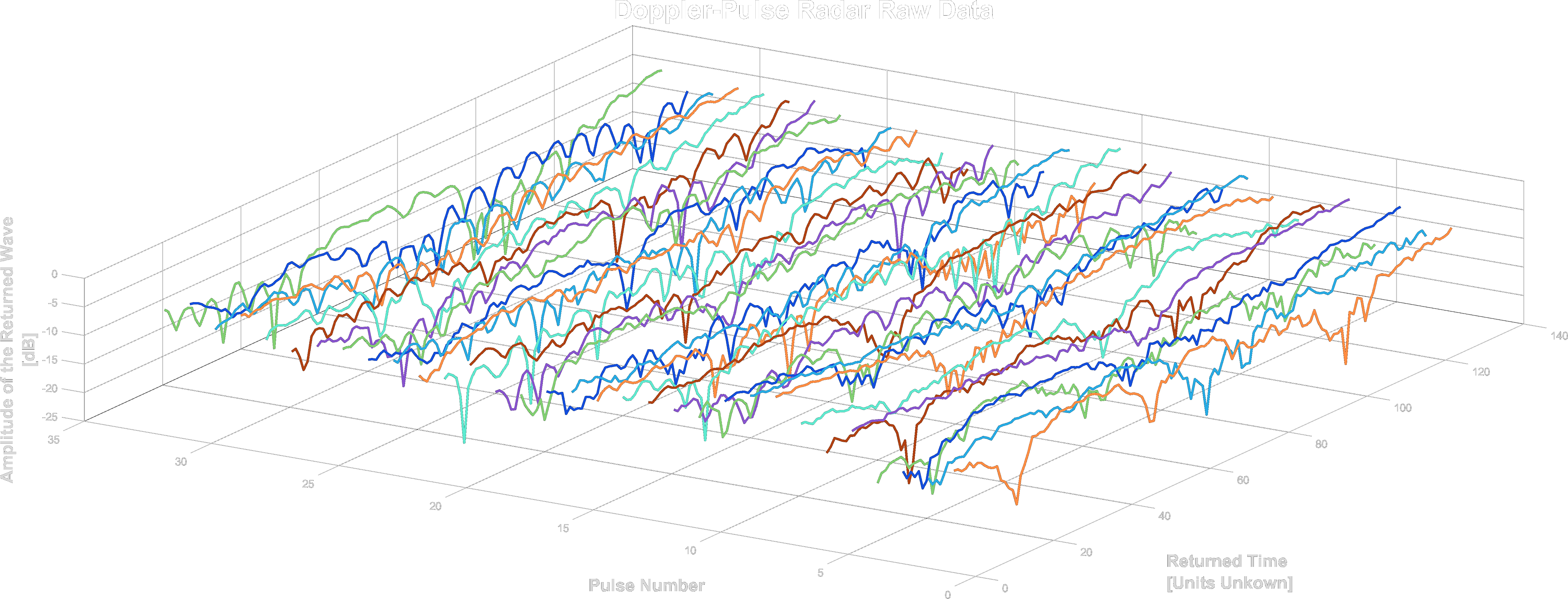
Example of a raw segment from the data, which was converted to power units. Each pulse was fired in “slow-time” intervals (32 times per segment).
Data & Dataset Structure
The metadata of a segment includes track id, location id, location type, day index, sensor id and the SNR level. The segments were collected from several different geographic locations, a unique id was given per location. Each location consists of one or more sensors, a sensor belongs to a single location. A unique id was given per sensor. Each sensor has been used in one or more days, each day is represented by an index. A single track appears in a single location, sensor and day. The segments were taken from longer tracks, each track was given a unique id.
The sets:
-
Training set: As the name describes, the training set consists of a combination of human and animal, with high and low SNR readings created from authentic doppler-pulse radar recordings.
(6656 Entries) -
Test set: For the purposes of the competition, a test set is included to evaluate the quality of the model and rank competitors. The set is unlabeled but does include a balanced mix of high and low SNR.
(106 Entries) -
Synthetic Low SNR set: Using readings from the training set a low SNR dataset has been artificially created by sampling the high SNR examples and artificially populating the samples with noise. This set can be used to better train the model on low SNR examples.
(50883 Entries) -
The Background set: The background dataset includes readings gathered from the doppler-pulse radars without specific targets. This set could be used to help the model better distinguish noise in the labelled datasets and help the model distinguish relevant information from messy data.
(31128 Entries) -
The Experiment set: The final set and possibly the most interesting, the experiment set includes humans recorded by the doppler-pulse radar in a controlled environment. Whilst not natural this could be valuable for balancing the animal-heavy training set provided.
(49071 Entries)
Submissions
In stage 1 we could submit, up to two times a day, the public test set. Submissions are evaluated on the Area Under the Receiver Operating Characteristic Curve (ROC AUC) between the predicted probability and the observed target. In the second stage, we could submit, up to two times total, the private test set.
My Strategy
My Tools
I only used my laptop for all the competition, it has an Nvidia GPU but with only 2GB of memory. Initially, I had 32GB of RAM but one of my sticks got fried from overtraining so I got stuck with 16GB of RAM close to the end (since there was a curfew so I could not have replaced it).
I mainly used MATLAB for testing different signal processing methods that will work well on the data. I used Python for implementing the signal processing methods I found and preprocess the data, train and test it using Keras models in TensorFlow.
Data Synthesization & Partition
It is important to ensure the data is balanced and unbiased as this can lead to significant misinterpretations of the set by the model, and small inconsistencies can get extrapolated into significant errors. Since the datasets are not balanced at all in categories like object(Human/Animal), SNR(High/Low), topography(Woods, Synthetic etc.) and the amount of data from each category is limited it was a challenge to find the right partition for the training and validation data.
For example, this is the code for the training dataset partition:
    geo1=((training_df["geolocation_id"]==1)&(training_df['segment_id'] % 4 == 0))#58
    geo2=((training_df["geolocation_id"]==2)&(training_df['segment_id'] % 3 == 0))#63
    geo3=((training_df["geolocation_id"]==3)&(training_df['segment_id'] % 16 == 0))#65
    geo4=((training_df["geolocation_id"]==4)&(training_df['segment_id'] % 3 == 0))#64
    train_NH_HS=((training_df["target_type"]!="human") & (training_df["snr_type"]=="HighSNR")&np.logical_not(geo1|geo2|geo3|geo4))
    train_NH_HS_val=((training_df["target_type"]!="human") & (training_df["snr_type"]=="HighSNR")&(geo1|geo2|geo3|geo4))#250

    geo1=((training_df["geolocation_id"]==1)&(training_df['segment_id'] % 4 == 0))#59
    geo2=((training_df["geolocation_id"]==2)&(training_df['segment_id'] % 1 == 0))#61
    geo3=((training_df["geolocation_id"]==3)&(training_df['segment_id'] % 57 == 0))#61
    geo4=((training_df["geolocation_id"]==4)&(training_df['segment_id'] % 5 == 0))#57
    train_NH_LS=((training_df["target_type"]!="human") & (training_df["snr_type"]=="LowSNR")&np.logical_not(geo1|geo2|geo3|geo4))#3.8k
    train_NH_LS_val=((training_df["target_type"]!="human") & (training_df["snr_type"]=="LowSNR")&(geo1|geo2|geo3|geo4))#238

    geo1=((training_df["geolocation_id"]==1)&(training_df['segment_id'] % 4 == 0))#111
    geo4=((training_df["geolocation_id"]==4)&(training_df['segment_id'] % 3 == 0))#123
    train_H_HS=((training_df["target_type"]=="human") & (training_df["snr_type"]=="HighSNR")&np.logical_not(geo1|geo4))#577
    train_H_HS_val=((training_df["target_type"]=="human") & (training_df["snr_type"]=="HighSNR")&(geo1|geo4))#234

    geo1=((training_df["geolocation_id"]==1)&(training_df['date_index'] % 3 == 0))#21
    geo4=((training_df["geolocation_id"]==4)&(training_df['segment_id'] % 3 == 0))#19
    train_H_LS=((training_df["target_type"]=="human") & (training_df["snr_type"]=="LowSNR")&np.logical_not(geo1|geo4))#48
    train_H_LS_val=((training_df["target_type"]=="human") & (training_df["snr_type"]=="LowSNR")&(geo1|geo4))#40

    train_idx=[]
    train_val_idx=[]
    if snr=="All" or snr=="Low":
        train_idx+=train_NH_LS+train_H_LS
        train_val_idx+=train_NH_LS_val+train_H_LS_val
    if snr=="All" or snr=="High":
        train_idx+=train_NH_HS+train_H_HS
        train_val_idx+=train_NH_HS_val+train_H_HS_val
Together with the rest of the partitions we get a balanced training and validation sets in terms of targets, SNR and geolocations.
I had to synthesize a new dataset to create new low SNR segments with animals. I added different noises, similar to the noise in other segments, to high SNR animal segments to create this new dataset.
Spectrograms
By going to the frequency domain using the Fourier Transform we can interpret the radar data quality easily.
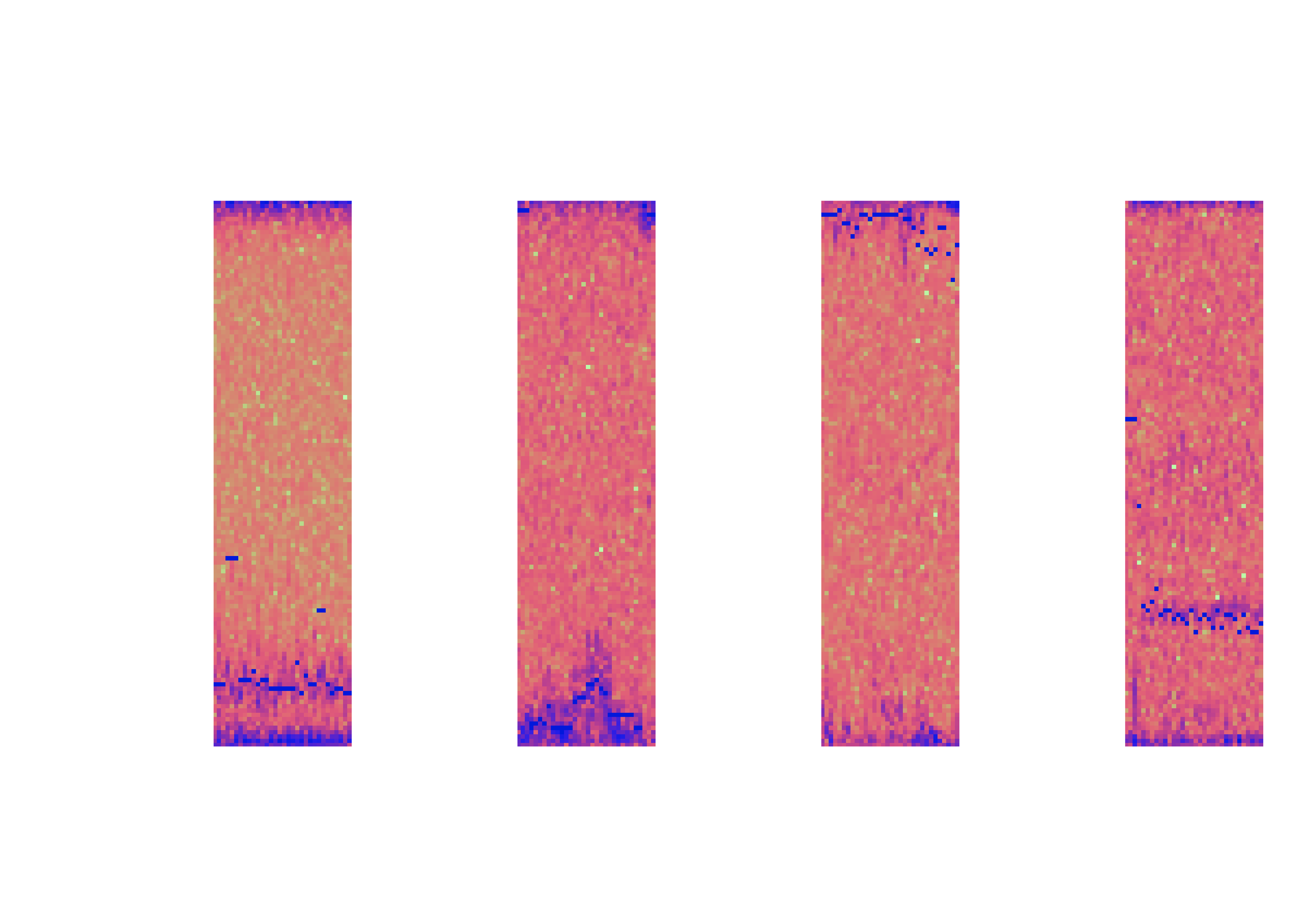
An example of the data included for the competition split by Animal/Human and High/Low Signal-Noise-Ratio. The I/Q matrices have been converted into spectrograms for visualization, and the target's doppler center-of-mass readings have been added as blue dots.
As you can see it’s not easy to identify the target only by the spectrogram (especially when units of measurement are not available), but using CNN we might detect patterns that are not easy to see.
Micro Doppler Effect
Since my rig was limited and training was taking days and I could not even use a relatively light model like ResNet50, I used my knowledge in Physics to look for an edge. The Doppler effect in this case is the shift in the light frequency due to the relative speed of the target. But targets that have motions relative to itself (or its centre of mass), like the rotation of the wheels on a car or the swinging of the hands when walking, create additional shifts in the light frequency that is called Micro-Doppler Effect.
Studding the MATLAB repository kozubv/doppler_radar I could simulate micro-Doppler effects that a human will create. First by creating a simulation of a human body walking:
A simulation of human body walking in MATLAB. The dots are the spots where the light will reflect from in the radar simulation.
And the resulting micro-Doppler effect spectrogram:
The resulting micro-Doppler effect spectrogram from the human walking simulation. The legitimates movement corresponds to the waves in the spectrogram.
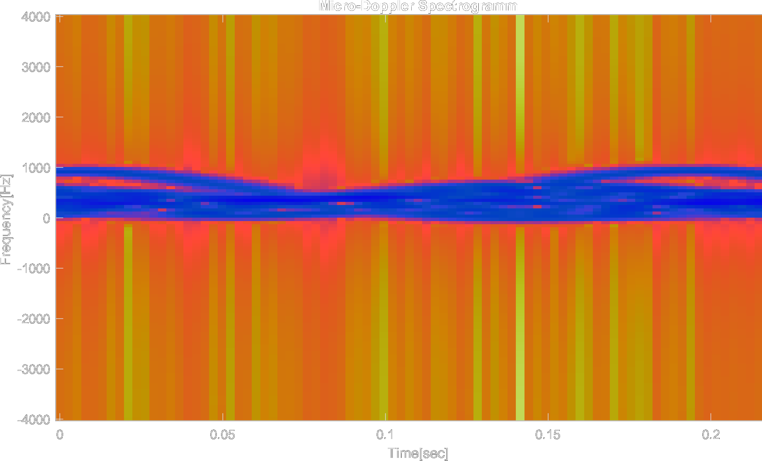
The extraction of the micro-Doppler spectrogram from the segments was a bit tricky since the segments only had 32 pulses to work with and not to mention the noise. Using different signal filters and windows I managed to get some decent results.
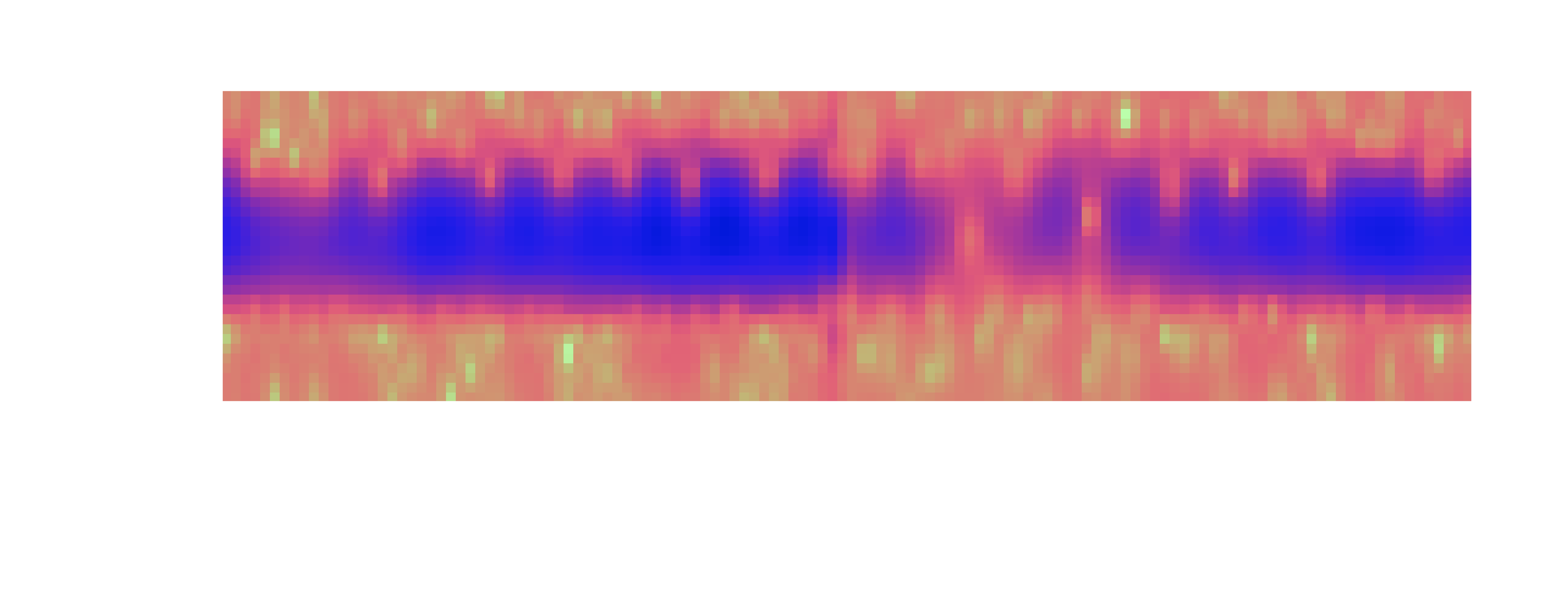
The resulting micro-Doppler spectrogram from a segment.
The Model
This part was a real challenge since I was really limited in the GPU department and had more than 20K segments in my training set (and around 3-4 different spectrograms per segment + other data). My computer couldn’t even use the ResNet50 for segments with one spectrogram. I combined knowledge from a dozen of articles that used spectrograms and micro-Doppler spectrograms to identify the object and other data to create a light but effective model architecture for this task. Initially, I used simple CNN as my model and over time I added more inputs and different layers. I ended up with merging two CNN models, one RNN and a simple NN. I input different low-res (to speed up learning) spectrograms to the CNN and took one of the micro-Doppler spectrograms and ran through the RNN (in the old days radar watcher could identify humans by the sound), I also included some neurones for data like SNR. Here is an example of one of the models I constructed:

An example of one of my models' architecture.
Results
I managed to receive around 90% accuracy (ROC_AUC) in the full public test and around 80% in the private test. I received the 30th place out of 1k+ participants including many companies like the Israel Air Industry(IAI) and Refael as well as research groups from universities. During the competition’s phase 1 there were attempts at cheating, my guess was that some people submitted a few random responses and via the score they managed to reproduce the correct data results. All in all, I’m happy with my results, not in my score (I know I could have done much better with a decent GPU and free time), but with the learning and the advance in experience I gained.
- Programmed in Python & MATLAB.
- Over 35K lines of code.This figure may include comment lines and some modified library files.
-
TensorFlow,
OpenCV,
NumPy,
Pandas,
Pillow,
SciPy, Matplotlib, Scikit-learn, Jupyter & Pickle used in Python.
| Lang/Lib/Pro | Version |
|---|---|
| MATLAB | R2020a |
| Python | 3.8.1 |
| TensorFlow | 2.3.0 |
| OpenCV | 4.3.0.36 |
| Jupyter | 6.1.6 |
| Matplotlib | 3.3.0 |
| NumPy | 1.18.5 |
| Scikit-learn | 0.23.1 |
| Pandas | 1.1.0 |
| Pillow | 7.1.2 |
| SciPy | 1.4.1 |
| Type | Python Scripts & Jupyter Notebooks |
| Input | Radar Raw Feed |
| Output | Classification |